For determining the timing, duration and temporal variability of environmental change, as recorded by palaeoenvironmental archives, ages based on optically stimulated luminescence (OSL) dating are superior to other approaches (e.g., ![]() C-dating). Moreover, luminescence dating is crucial for time scale construction for considerable parts of the Quaternary, since it captures the depositional process of sediment itself. For an introduction to luminescence dating see e.g., Aitken (1998) or Preusser et al. (2008). One step beyond interpreting particular depositional ages is deploying chronologies using multiple ages in any succession of deposited sediment, i.e., converting the depth or thickness domain of a deposit to the time domain, commonly referred to as age-depth-model. Numerical chronologies represent a defined transformation of stratigraphic positions/layers to time in Earth's history, giving a fundamental basis for most studies on palaeoenvironments. Age-depth-models can be constructed by linear interpolation or fitting of polynomial or spline functions to existing ages. More sophisticated Bayesian models, in the sense of allowing statistical inferences using probability models, allow for obtaining robust age-depth-models by incorporating uncertainties from sets of individual dates (e.g., Buck et al., 1991, 1992; Bronk Ramsey, 1995; Bayliss and Ramsey, 2004; Blaauw and Christen, 2011; Blaauw and Heegaard, 2012), and sometimes also assumptions on the depositional processes (Bronk Ramsey, 2009). In particular, this involves obtaining additional information inherent to the stratigraphic sequence, i.e., by applying the stratigraphic principle that deposits lower in the profile sequence are presumably older than shallower ones. The application of Bayesian methods to stratigraphies, which are in detail described in, e.g., Bronk Ramsey, (1995, 2000, 2001) and Buck et al., (1996), reduce the uncertainty of datasets with known chronological order where age probability density functions (PDF) overlap. Most commonly, this approach uses Markov Chain Monte Carlo (MCMC) simulations (cf. Gelman et al., 2014 for an introduction). Bronk Ramsey (2000, 2009) and Steier and Rom (2000) demonstrate the relevance of depositional system assumptions and specifically Bronk Ramsey (2000) points out that the results strictly represent results of applied methods. Telford et al (2004) and Blockley et al (2007) demonstrate that age-depth-models may give misleading accuracy when the spatial distance of dated layers is not small enough. It becomes generally accepted that Bayesian age models including reproducible uncertainty are more realistic than models without uncertainty estimation (Blaauw, 2010).
In the past, Bayesian age modelling approaches were mainly used by the
C-dating). Moreover, luminescence dating is crucial for time scale construction for considerable parts of the Quaternary, since it captures the depositional process of sediment itself. For an introduction to luminescence dating see e.g., Aitken (1998) or Preusser et al. (2008). One step beyond interpreting particular depositional ages is deploying chronologies using multiple ages in any succession of deposited sediment, i.e., converting the depth or thickness domain of a deposit to the time domain, commonly referred to as age-depth-model. Numerical chronologies represent a defined transformation of stratigraphic positions/layers to time in Earth's history, giving a fundamental basis for most studies on palaeoenvironments. Age-depth-models can be constructed by linear interpolation or fitting of polynomial or spline functions to existing ages. More sophisticated Bayesian models, in the sense of allowing statistical inferences using probability models, allow for obtaining robust age-depth-models by incorporating uncertainties from sets of individual dates (e.g., Buck et al., 1991, 1992; Bronk Ramsey, 1995; Bayliss and Ramsey, 2004; Blaauw and Christen, 2011; Blaauw and Heegaard, 2012), and sometimes also assumptions on the depositional processes (Bronk Ramsey, 2009). In particular, this involves obtaining additional information inherent to the stratigraphic sequence, i.e., by applying the stratigraphic principle that deposits lower in the profile sequence are presumably older than shallower ones. The application of Bayesian methods to stratigraphies, which are in detail described in, e.g., Bronk Ramsey, (1995, 2000, 2001) and Buck et al., (1996), reduce the uncertainty of datasets with known chronological order where age probability density functions (PDF) overlap. Most commonly, this approach uses Markov Chain Monte Carlo (MCMC) simulations (cf. Gelman et al., 2014 for an introduction). Bronk Ramsey (2000, 2009) and Steier and Rom (2000) demonstrate the relevance of depositional system assumptions and specifically Bronk Ramsey (2000) points out that the results strictly represent results of applied methods. Telford et al (2004) and Blockley et al (2007) demonstrate that age-depth-models may give misleading accuracy when the spatial distance of dated layers is not small enough. It becomes generally accepted that Bayesian age models including reproducible uncertainty are more realistic than models without uncertainty estimation (Blaauw, 2010).
In the past, Bayesian age modelling approaches were mainly used by the ![]() C community (e.g., Bayliss and Ramsey, 2004; Millard, 2004), but have also been applied to archaeomagnetism (Lanos et al., 2005; Schnepp and Lanos, 2005), U/Pb dating (Mundil, 2004; de Vleeschouwer and Parnell, 2014;), U-series dating of speleothems (Millard, 2004; Scholz and Hoffmann, 2011; Hercman and Pawlak, 2012), ESR dating (Millard, 2006a), 210Pb dating (Hercman et al., 2014) and to the integration of
C community (e.g., Bayliss and Ramsey, 2004; Millard, 2004), but have also been applied to archaeomagnetism (Lanos et al., 2005; Schnepp and Lanos, 2005), U/Pb dating (Mundil, 2004; de Vleeschouwer and Parnell, 2014;), U-series dating of speleothems (Millard, 2004; Scholz and Hoffmann, 2011; Hercman and Pawlak, 2012), ESR dating (Millard, 2006a), 210Pb dating (Hercman et al., 2014) and to the integration of ![]() Ar/
Ar/![]() Ar ages and cyclostratigraphic durations (Meyers et al., 2012; Sageman et al., 2014). Luminescence ages have been used for Bayesian age modelling, as well (Rhodes et al., 2003; Millard, 2004, 2006b; Huntriss, 2008; Combès and Philippe, 2017), but so far this procedure received only limited attention. Millard (2004) comments on the rare use of Bayesian age models applied to other dating techniques than
Ar ages and cyclostratigraphic durations (Meyers et al., 2012; Sageman et al., 2014). Luminescence ages have been used for Bayesian age modelling, as well (Rhodes et al., 2003; Millard, 2004, 2006b; Huntriss, 2008; Combès and Philippe, 2017), but so far this procedure received only limited attention. Millard (2004) comments on the rare use of Bayesian age models applied to other dating techniques than ![]() C and states: ``The beauty of Bayesian chronological models is their ability to combine many different types of information in a mathematically rigorous and philosophically satisfying way. It is natural therefore to extend the method to the other available dating techniques``.
C and states: ``The beauty of Bayesian chronological models is their ability to combine many different types of information in a mathematically rigorous and philosophically satisfying way. It is natural therefore to extend the method to the other available dating techniques``.
This limited use of Bayesian age model improvement by other dating techniques may be related to the difficulties in providing a separation of the systematic and random parts of uncertainty. Only the random uncertainty part can be used for modelling (e.g., Gradstein et al., 2004; Huntriss, 2008; Agterberg et al., 2012). Here we consider samples from individual sediment sections measured in the same laboratory and their uncertainty parts. We regard uncertainty as random, when it does not bias ages in a systematic manner towards older or younger ages. Luminescence data can be expected to gain improved precision by Bayesian methods due to its comparably high uncertainty and often overlapping probability density functions. Combinations of systematic and random uncertainty may be expected in all dating methods. Comparing datasets of different luminescence techniques (e.g., Kreutzer et al., 2012; Constantin et al., 2014; Lomax et al., 2014; Trandafir et al., 2015) are examples where both systematic and random uncertainty structures are present. For routine dating applications, the parts of uncertainty have so far not been separated in a reproducible way.
Various software packages implement Bayesian age models, specifically for ![]() C dating, such as OxCal (e.g., Bronk Ramsey, 1995) and ChronoModel (Vibet et al., 2016). Simulations using age distributions are employed to obtain datasets consistent with the stratigraphic principle. However, only random uncertainty should be used in such models, and model results need to be re-combined with the systematic part of uncertainty after modelling. The necessity for separating uncertainty into random and systematic parts and attempts from a physical understanding are discussed already in Aitken, (1985), but due to the unknown uncertainty structure of several parameters of the age equation (e.g., the water content which contributes significant to uncertainty) all physical models remain rough approximations.
C dating, such as OxCal (e.g., Bronk Ramsey, 1995) and ChronoModel (Vibet et al., 2016). Simulations using age distributions are employed to obtain datasets consistent with the stratigraphic principle. However, only random uncertainty should be used in such models, and model results need to be re-combined with the systematic part of uncertainty after modelling. The necessity for separating uncertainty into random and systematic parts and attempts from a physical understanding are discussed already in Aitken, (1985), but due to the unknown uncertainty structure of several parameters of the age equation (e.g., the water content which contributes significant to uncertainty) all physical models remain rough approximations.
Scope of this article is to introduce an inverse modelling approach to resolve the proportions of systematic and random uncertainty for sets of luminescence ages from individual sections. We focus on one type of terrestrial archive (Late Quaternary loess-palaeosol-sequences) and one type of luminescence dating technique (fine-grain quartz based OSL). Based on a database of published records, a PDF of the random uncertainty is created and an existing chronology is exemplary improved. The approach is validated with synthetic data sets of known composition and applied to an empiric data set from Saxony/Germany (Kreutzer et al., 2012). The power of the here proposed method is to work even without knowing the sources of uncertainty, the means of obtaining them, and their correlation. This approach may be considered rough, but at the same time it is effective when only age results are known. This is inevitably the case if original data sets are not available.
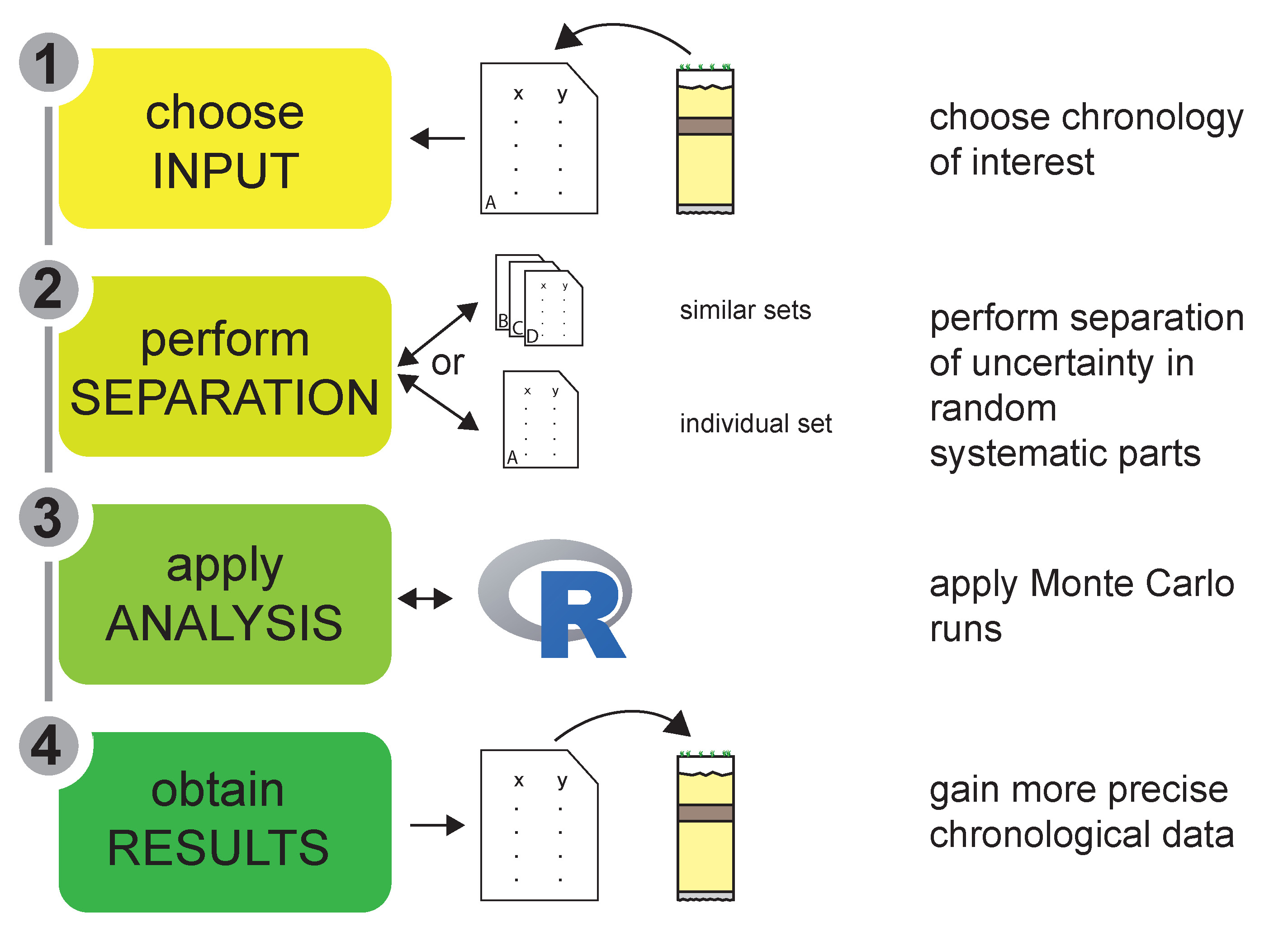
The approach consists of three parts (Fig. 1). First, a survey of published OSL chronology data sets for loess-palaeosol-sequences is integrated to a database of appropriate material. Second, based on this OSL data a PDF of the random uncertainties is generated, applying MCMC methods, using resampling statistics. A PDF is preferred here to a fixed value of random/systematic uncertainty, as these may be different for individual ages from a dataset. Third, this PDF-based information about the random uncertainties is used in a Bayesian age-depth model to calculate more precise ages with reduced combined uncertainties. All calculations are programmed and performed using the free statistic programming language R (R Development Core Team, 2017). The two models (PDF generation and age recalculation) are written as documented functions and - together with test data sets - provided as Appendix and supplementary data repository for reproduction and modification of the results reported here. Please note that our calculations using resampling procedures; hence results vary for different experiments and may not be perfectly reproducible. Throughout this text R code snippets or function arguments are given in monospaced characters and refer to full R code provided in the supplementary material.
Separation of random and systematic uncertainty parts of OSL data requires a robust and sufficiently large database of dated sediment deposits. Deposits have to be stratigraphically consistent and must unambiguously allow an identification of age inversions from, e.g., morphological features of the deposits. The sediment transport process that generated the deposit should allow for well-bleached sediments prior to burial (e.g., due to atmospheric suspension transport) and should show minimal post-depositional disturbance. Accordingly, to build the empiric database we focus on OSL ages reported for well documented (mainly European) loess and loess-palaeosol sequences that show high accumulation rates, especially during the last glacial maximum (Rousseau et al., 2007; Buggle et al., 2009; Újvári et al., 2010). Furthermore, aeolian sediments can be expected as sufficiently bleached before deposition.
The selection of the datasets was based on a series of rigorous constraints: (1) Only OSL age estimates obtained by fine grain (4-11 ![]() m) quartz dating using the single aliquot regenerative-dose (SAR) approach (Murray and Wintle, 2000) are considered, (2) ages showing an equivalent dose (D
m) quartz dating using the single aliquot regenerative-dose (SAR) approach (Murray and Wintle, 2000) are considered, (2) ages showing an equivalent dose (D![]() ) higher than 150 Gy are neglected (equivalent to a maximum age of about 50 ka in a loess section, depending on the environmental radioactivity), (3) only records with limited pedogenic disturbances are used. The first constraints are introduced to avoid dealing with systematic methodological uncertainties that may not be comparable, and may not be fully understood from a physical perspective. Setting a cut-off level for D
) higher than 150 Gy are neglected (equivalent to a maximum age of about 50 ka in a loess section, depending on the environmental radioactivity), (3) only records with limited pedogenic disturbances are used. The first constraints are introduced to avoid dealing with systematic methodological uncertainties that may not be comparable, and may not be fully understood from a physical perspective. Setting a cut-off level for D![]() at 150 Gy is somewhat arbitrary and a balance between data availability and suggested higher reliability of lower D
at 150 Gy is somewhat arbitrary and a balance between data availability and suggested higher reliability of lower D![]() values. The mineral quartz was chosen because it is supposed not to suffer from an anomalous signal loss over time (athermal fading, an effect that leads to age underestimation; Wintle, 1973). Further, the limitation to D
values. The mineral quartz was chosen because it is supposed not to suffer from an anomalous signal loss over time (athermal fading, an effect that leads to age underestimation; Wintle, 1973). Further, the limitation to D![]() values < 150 Gy accounts for the reported and expected dose saturation levels of quartz in general, which range from about 125 Gy up to about 400 Gy in exceptional cases (cf. Buylaert et al., 2007; Roberts, 2008; Chapot et al., 2012). This limit is kept for all datasets; even when a study reported locally higher saturation levels.
values < 150 Gy accounts for the reported and expected dose saturation levels of quartz in general, which range from about 125 Gy up to about 400 Gy in exceptional cases (cf. Buylaert et al., 2007; Roberts, 2008; Chapot et al., 2012). This limit is kept for all datasets; even when a study reported locally higher saturation levels.
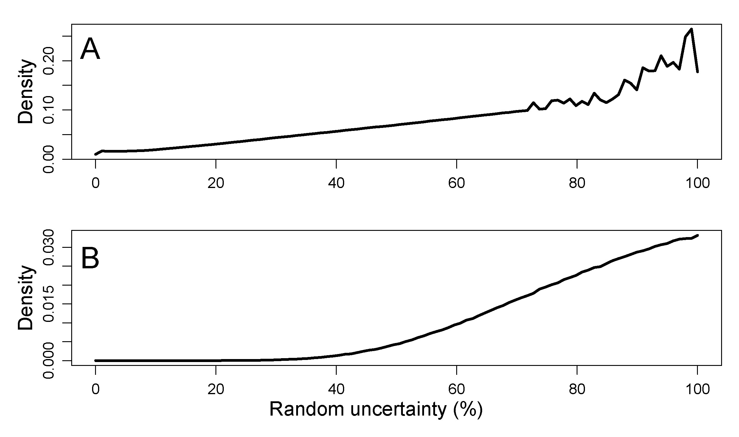
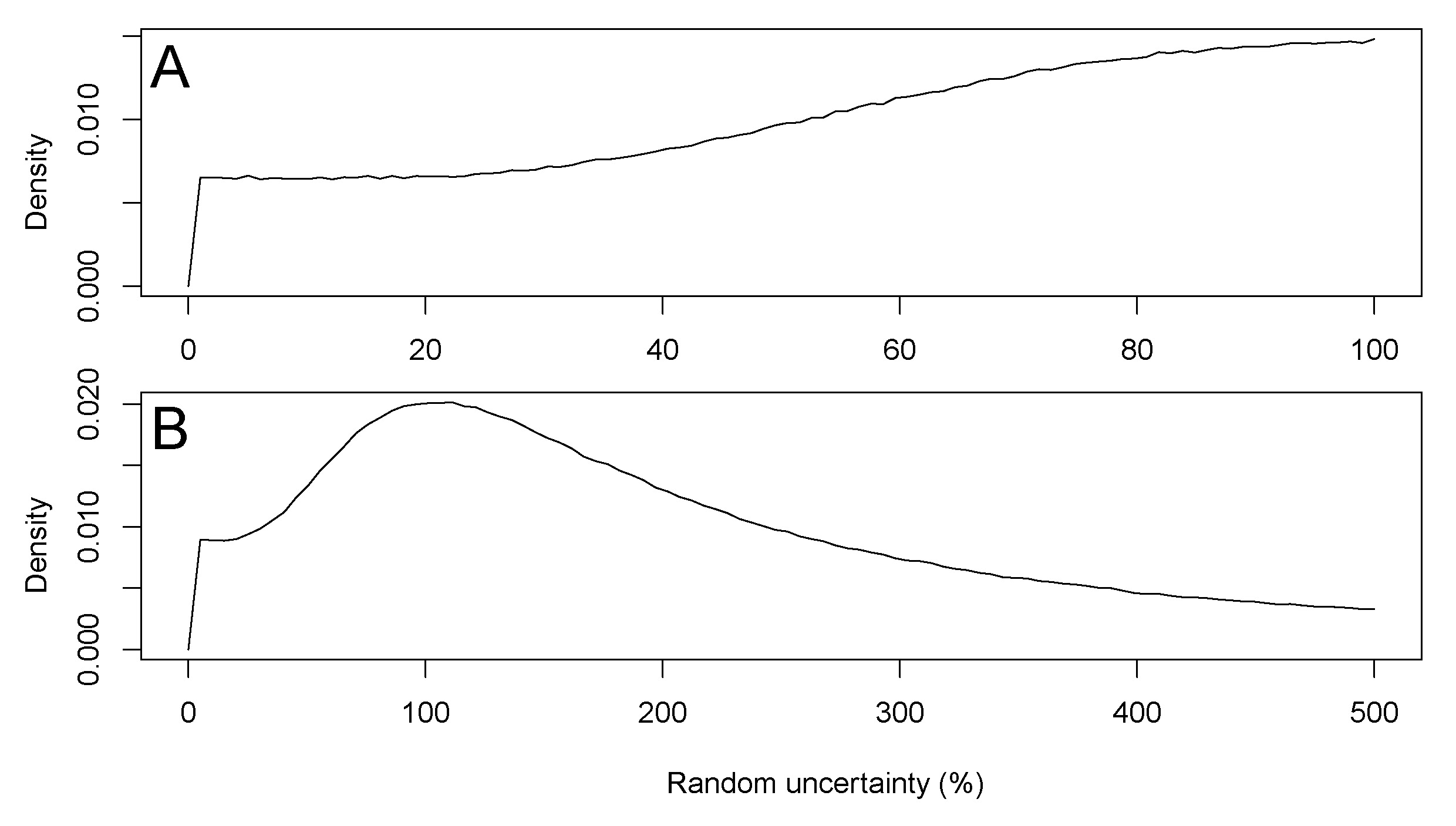
When investigating sediment samples with a similar source area and deposition history, age inversions within a concordant sediment section may be explained at first order by the random uncertainty of a dating method. Any dating method with inherent random uncertainty is expected to show age inversions. Thereby, the number of inversions should only depend on the proportion of random uncertainty for the dated samples, whereas systematic uncertainty causes bias in one direction (old/young) and does not contribute to age inversions. To create a synthetic record with imposed uncertainty, ages of datasets are ordered. Accordingly, for each data set random uncertainties, ranging from 1 % to 100 % (and systematic uncertainties vice versa) are tested for their ability to explain the observed number of age inversions. The tests included for each combination of uncertainty parts, realised as a sequence of integer percentages of random uncertainty (n = 100), 1001 times (n.MC = 1001) resampling the natural dataset with the given uncertainty properties. All random uncertainty parts that could explain the empiric number of age inversions were given a relative probability, representing a measure for the number of simulations in agreement with real luminescence data and their number of inversions (Fig. 2). Fig. 2A depicts the PDF for all here considered datasets, and Fig. 2B represents the PDF from a single dataset by Kreutzer et al. (2012). The function create.pdf uses datasets and their 1-sigma uncertainty as input, because most datasets are published with this uncertainty level. In summary, we test different amounts of random uncertainty (in %) for their possibility to create the number of observed age inversions. This is done using simulations of reported ages and their uncertainty. Noisy PDFs can be result of sparse simulation cases consistent with data, and also unclear density due to a limited number of simulations. In some cases, this can be countered by increasing the number of simulations where computer memory allows.
|
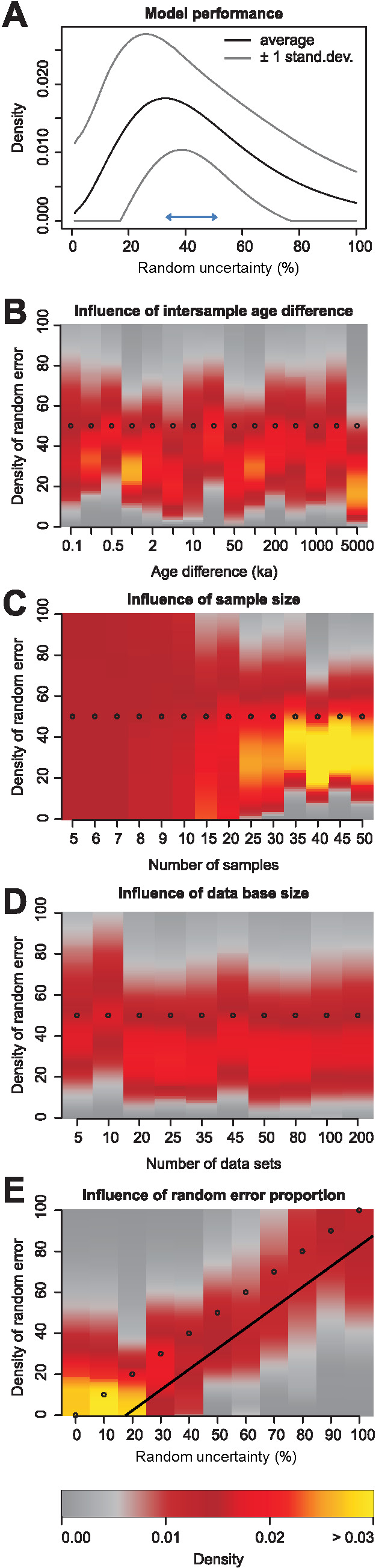
Synthetic data sets are created to explore the validity and performance of the uncertainty separation algorithm. Questions to be addressed concern the influence of the number of samples in a dataset, the number of different data sets, the proximity of individual ages to each other and the overall size of the relative uncertainty on the shape of the random uncertainty density function. The supplementary materials contain a series of R-scripts that are devoted resolving these questions and may be used by the reader to comprehend and extend the tests (Fig. 3).
|
To estimate the overall scatter introduced by the technique, a Monte Carlo design with 500 repeated simulations of one data set with 35 samples was created. The samples in this data set are all separated by 500 years, starting from zero, have a relative uncertainty of 12 % and a random uncertainty part of 50 %. Based on these parameters, in each Monte Carlo run normal distributed random numbers were generated with the means defined by the evenly spaced ages and the standard deviations defined by the random uncertainty parts of the relative uncertainty.
To test the influence of age offsets within a chronology (i.e., effect of sampling density or deposition rate; see Fig. B, Supplementary script 04_test_age_offset.R), the spacing of individual ages was changed from 5 years to 50,000 years. The limits of this range are far from being realistically encountered in any empiric data set but highlight the behaviour of the algorithm also in extreme cases. To test the influence of the sample size, their number in a data set was changed from 5 to 50 (logarithmically increasing; see Fig. 3C and Supplementary script 05_test_number_of_samples.R). The upper limit of this range will be encountered only in few empiric data sets and is primarily used to show the influence of this parameter. The influence of number of empiric data sets (i.e., size of the data base; see Fig. 3D and Supplementary script 06_test_number_of_data_sets.R) was tested by changing the data base size from 5 to 200. In a last test, the relative uncertainty was changed from 0 % to 100 % in integer steps to test the influence of this parameter; see Fig. 3E and Supplementary script 07_test_random_uncert_part.R.
Buck et al. (1991) introduced the consideration of the principle of stratigraphy in a statistical way to ![]() C dating, and the concept has been described in detail various times thereafter (e.g., Buck et al., 1991, 1992; Bronk Ramsey, 1995; 2000; Steier and Rom, 2000; Blockley et al., 2004). Here, the PDF as derived from the empirical data set is used to generate random uncertainty parts and assign them to a series of empiric ages in stratigraphic order. The respective systematic uncertainty part is stored separately and is not used for the following age-depth modelling procedure, but is re-combined with the final result. This procedure is applied to in total as many simulation runs as necessary to gain
C dating, and the concept has been described in detail various times thereafter (e.g., Buck et al., 1991, 1992; Bronk Ramsey, 1995; 2000; Steier and Rom, 2000; Blockley et al., 2004). Here, the PDF as derived from the empirical data set is used to generate random uncertainty parts and assign them to a series of empiric ages in stratigraphic order. The respective systematic uncertainty part is stored separately and is not used for the following age-depth modelling procedure, but is re-combined with the final result. This procedure is applied to in total as many simulation runs as necessary to gain n.MC.min (default:1000) stratigraphically consistent data sets. The routine recalculate.ages estimates the number of required MCMC runs based on a subsample size and improves computational efficiency through vectorisation of the calculations in R. Depending on the likelihood to draw inverted ages from the input data description, this can involve a large number of Monte Carlo runs, which are cut by a parameter n.MC.max to avoid longer than necessary processing. The recalculate.ages routine uses the 2-sigma uncertainty of data as input, and by default provides 95 % uncertainty of the Bayesian model result; the output probabilities can be set by adjusting the probability parameter. It calculates a maximum of n.MC.max times n.MC.min simulations.
Straightforward interpretation of resulting simulations with stratigraphically consistent data are problematic (cf. Bronk Ramsey, 2000, 2009; Steier and Rom, 2000). Uncorrected results from MCMC simulations have a higher probability for results with relatively long durations exceeding means of original maximum and minimum ages (and producing datasets with youngest ages shifted towards younger ages, and the oldest age being shifted towards the older end). To account for this effect, the Bayesian weighting prior for ordered data sets is defined according to (Bronk Ramsey, 2000, 2009):
![]() , where tmax is the oldest sample age, tmin the youngest sample age and n is the number of ages/samples, including the introduction of two boundary ages to counter effects of preferring long durations (e.g., Bronk Ramsey, 2000). For unordered datasets P was set to 0, as outlined, e.g., in Bronk Ramsey (2000). Furthermore, two outer boundary ages are set at a distance of five times the mean temporal spacing of samples (similar to boundaries in OxCal; Bronk Ramsey, 2009). Fig. 4 shows how the applied algorithm avoids preferring long durations and successfully accounts for this issue.
, where tmax is the oldest sample age, tmin the youngest sample age and n is the number of ages/samples, including the introduction of two boundary ages to counter effects of preferring long durations (e.g., Bronk Ramsey, 2000). For unordered datasets P was set to 0, as outlined, e.g., in Bronk Ramsey (2000). Furthermore, two outer boundary ages are set at a distance of five times the mean temporal spacing of samples (similar to boundaries in OxCal; Bronk Ramsey, 2009). Fig. 4 shows how the applied algorithm avoids preferring long durations and successfully accounts for this issue.
|
However, this effect may affect results from other datasets with other data structures. Specifically, the pattern of inversions and age non-equidistant distance between samples (or clustering of samples at specific age intervals) may influence this effect. Summarizing, the re-calculation of OSL ages represents an age-depth model using the mentioned Bayesian Prior and a PDF of the random and systematic parts of uncertainty.
Results from 500 repeated model-runs with identical input parameters show a high probability density between 25 % and 40 % random uncertainty (maximum around a random uncertainty of 35 %). These results imply an underestimation of the true random uncertainty part by 10 % to 25 % (18 % on average, cf. Figs. 3a (see the peak at 38 % instead of 50 %, indicated by the arrow), 3e (see colours representing high density systematically below the 50 % dots, the line indicates the 18 % lowered density), and supplementary materials). The density curve is asymmetric with a negative skew. Age differences between samples do not influence the model results (Fig. 3B). The rather stable underestimate of about 18 % is observed regardless of the age difference between samples, and thus the potentially existing age inversions due to random uncertainty (see specifically Fig. 3A & 3E). Sample size has a significant impact on model results (Fig. 3c). With less than about 10 samples per dataset the PDF is rather flat. It indicates basically any proportions of random and systematic uncertainty are equally likely. From about 15 samples onward, the PDF becomes systematically narrower. However, even as many as 50 samples do not influence the observed underestimation. The size of a data base (i.e., the number of individual datasets) does not influence the model results. Despite the about 18 % underestimation effect our approach reliably detects all imposed random uncertainty proportions (Fig. 3e).
Data regarded reliable by the authors and fulfilling the criteria outlined in section 2.1 are contained in publications by ChongYi et al., 2012; Constantin et al., 2014, 2015; Fuchs et al., 2013; Kreutzer et al., 2012; Lu et al., 2007 (one age fulfills criteria but is not regarded as robust by the authors); Meszner et al., 2013; Timar-Gabor et al., 2011. For unknown reasons the dataset by Meszner et al., (2013) suggests random uncertainty to largely exceed the overall uncertainty (see supplementary Fig. 1). Thus, we excluded this dataset from further analysis. These sets were used to create a PDF for fine grain OSL ages of the sediment type loess. The empiric PDF (PDF![]() , Table 1, Fig. 2a) reveals that high percentages of random uncertainty have a higher probability than low percentages of random uncertainty. The PDF generated from all input data sets, hereafter termed ''PDF
, Table 1, Fig. 2a) reveals that high percentages of random uncertainty have a higher probability than low percentages of random uncertainty. The PDF generated from all input data sets, hereafter termed ''PDF![]() ``, shows an almost linearly increasing probability for higher contributions of random uncertainty. Applying the approach to a single data set (Kreutzer et al., 2012) yields different results (Fig. 2b). There, the PDF has the highest probability for high random uncertainty percentages and declines with lower values. The PDF approaches zero for values smaller than about 30 % random uncertainty.
``, shows an almost linearly increasing probability for higher contributions of random uncertainty. Applying the approach to a single data set (Kreutzer et al., 2012) yields different results (Fig. 2b). There, the PDF has the highest probability for high random uncertainty percentages and declines with lower values. The PDF approaches zero for values smaller than about 30 % random uncertainty.
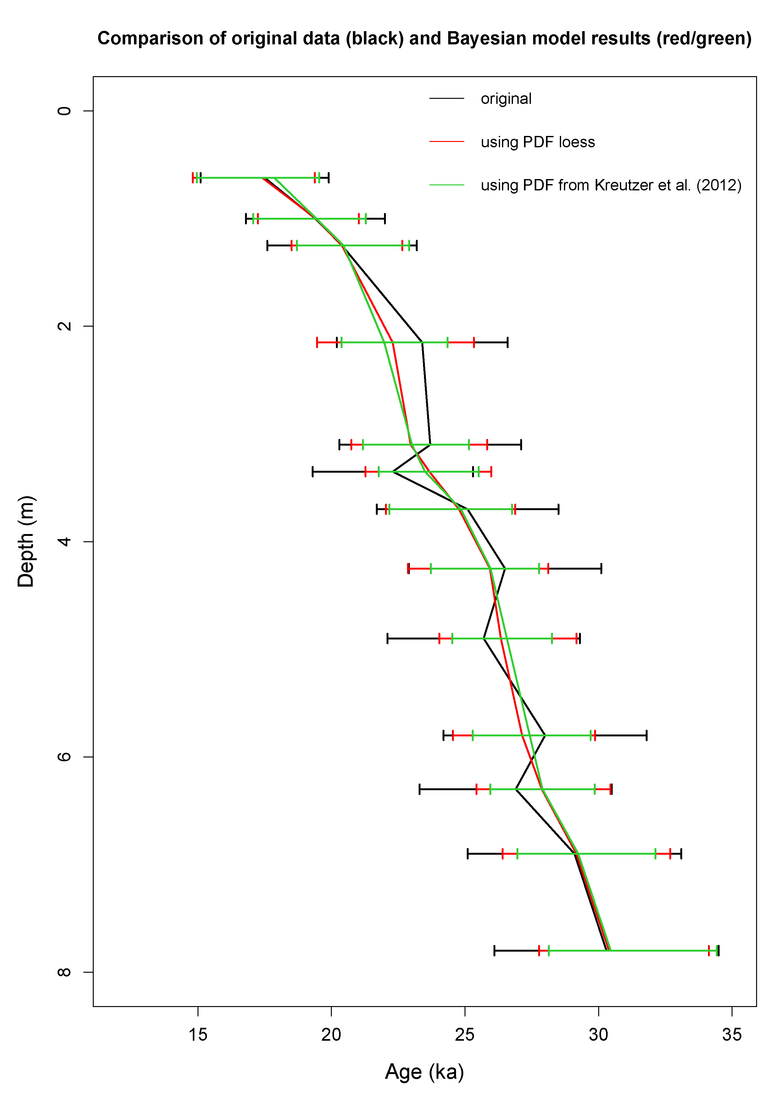
Results of the original and refined chronologies of the empiric data set from Ostrau/Saxony (Kreutzer et al., 2012, Fig. 4) reveal that the overall uncertainty of the data could be reduced on average by 30 % when using the PDF from this specific dataset, and by 21 % when using the PDF from all input data sets (PDF![]() ; Table1). The improvement is expressed as the difference between the uncertainty after modelling and the original uncertainty over the original uncertainty (all 2-sigma). Data near the top and bottom of the sediment section cannot be improved to a similar extent as data in between (Table 2 and Fig. 4).
; Table1). The improvement is expressed as the difference between the uncertainty after modelling and the original uncertainty over the original uncertainty (all 2-sigma). Data near the top and bottom of the sediment section cannot be improved to a similar extent as data in between (Table 2 and Fig. 4).
| uncertainty [%] | probability | uncertainty [%] | probability | uncertainty [%] | probability |
| 0 | 0.01000628 | 33.333333 | 0.04821316 | 66.666667 | 0.09243584 |
| 1.010101 | 0.016541 | 34.343434 | 0.04934387 | 67.676768 | 0.09411864 |
| 2.020202 | 0.01645952 | 35.353535 | 0.05076916 | 68.686869 | 0.09503695 |
| 3.030303 | 0.01645641 | 36.363636 | 0.05197299 | 69.69697 | 0.09674894 |
| 4.040404 | 0.01644975 | 37.373737 | 0.05350727 | 70.707071 | 0.09791893 |
| 5.050505 | 0.01644684 | 38.383838 | 0.0543716 | 71.717172 | 0.09893429 |
| 6.060606 | 0.0167408 | 39.393939 | 0.05586333 | 72.727273 | 0.11468022 |
| 7.070707 | 0.01720838 | 40.40404 | 0.05712714 | 73.737374 | 0.10165718 |
| 8.080808 | 0.01769127 | 41.414141 | 0.05872534 | 74.747475 | 0.1027008 |
| 9.090909 | 0.01850702 | 42.424242 | 0.05997554 | 75.757576 | 0.11876968 |
| 10.10101 | 0.01949214 | 43.434343 | 0.06107018 | 76.767677 | 0.11997022 |
| 11.111111 | 0.02069329 | 44.444444 | 0.06266646 | 77.777778 | 0.11389758 |
| 12.121212 | 0.02177999 | 45.454545 | 0.06405702 | 78.787879 | 0.12238049 |
| 13.131313 | 0.02283053 | 46.464646 | 0.06540718 | 79.79798 | 0.10880839 |
| 14.141414 | 0.02402877 | 47.474747 | 0.06628864 | 80.808081 | 0.1175924 |
| 15.151515 | 0.02512093 | 48.484848 | 0.06753321 | 81.818182 | 0.11098616 |
| 16.161616 | 0.02631646 | 49.494949 | 0.06883373 | 82.828283 | 0.13406463 |
| 17.171717 | 0.02733976 | 50.505051 | 0.07050314 | 83.838384 | 0.12053686 |
| 18.181818 | 0.02867175 | 51.515152 | 0.07177392 | 84.848485 | 0.1149341 |
| 19.191919 | 0.02969268 | 52.525253 | 0.07315606 | 85.858586 | 0.12210364 |
| 20.20202 | 0.03105637 | 53.535354 | 0.07441017 | 86.868687 | 0.13114198 |
| 21.212121 | 0.03223179 | 54.545455 | 0.07580185 | 87.878788 | 0.16076203 |
| 22.222222 | 0.03365747 | 55.555556 | 0.07761307 | 88.888889 | 0.15430351 |
| 23.232323 | 0.03498134 | 56.565657 | 0.07876972 | 89.89899 | 0.14087445 |
| 24.242424 | 0.03605716 | 57.575758 | 0.08015879 | 90.909091 | 0.18570389 |
| 25.252525 | 0.0375575 | 58.585859 | 0.08125125 | 91.919192 | 0.17900544 |
| 26.262626 | 0.03893187 | 59.59596 | 0.08261136 | 92.929293 | 0.17969401 |
| 27.272727 | 0.03998447 | 60.606061 | 0.08435207 | 93.939394 | 0.20995126 |
| 28.282828 | 0.04152177 | 61.616162 | 0.08569958 | 94.949495 | 0.18861811 |
| 29.292929 | 0.04302369 | 62.626263 | 0.08709216 | 95.959596 | 0.19655025 |
| 30.30303 | 0.044297 | 63.636364 | 0.08836269 | 96.969697 | 0.18295683 |
| 31.313131 | 0.04546706 | 64.646465 | 0.08982048 | 97.979798 | 0.24858113 |
| 32.323232 | 0.04657738 | 65.656566 | 0.09097122 | 98.989899 | 0.26420855 |
| Original data | PDF of all loess datasets | PDF Kreutzer et al. (2012) data | ||||||||
| sample | Depth | Age | 1 |
2 |
mean age | lower |
upper |
mean age | lower |
upper |
| boundary | ||||||||||
| BT607 | 0.15 | 15.1 | 1.4 | 2.8 | 15.01 | 12.10 | 17.71 | 15.23 | 11.44 | 18.00 |
| BT608 | 0.62 | 17.5 | 1.2 | 2.4 | 17.41 | 14.81 | 19.38 | 17.86 | 14.96 | 19.54 |
| BT609 | 1 | 19.4 | 1.3 | 2.6 | 19.43 | 17.25 | 21.03 | 19.44 | 17.08 | 21.29 |
| BT610 | 1.25 | 20.4 | 1.4 | 2.8 | 20.40 | 18.51 | 22.66 | 20.45 | 18.71 | 22.91 |
| BT611 | 2.15 | 23.4 | 1.6 | 3.2 | 22.29 | 19.47 | 25.33 | 21.98 | 20.38 | 24.35 |
| BT612 | 3.1 | 23.7 | 1.7 | 3.4 | 22.97 | 20.75 | 25.83 | 23.02 | 21.18 | 25.15 |
| BT613 | 3.35 | 22.3 | 1.5 | 3 | 23.67 | 21.28 | 25.98 | 23.51 | 21.77 | 25.52 |
| BT614 | 3.7 | 25.1 | 1.7 | 3.4 | 24.78 | 22.04 | 26.88 | 24.85 | 22.17 | 26.76 |
| BT615 | 4.25 | 26.5 | 1.8 | 3.6 | 25.93 | 22.87 | 28.12 | 25.96 | 23.73 | 27.78 |
| BT616 | 4.9 | 25.7 | 1.8 | 3.6 | 26.35 | 24.04 | 29.18 | 26.57 | 24.53 | 28.26 |
| BT626 | 5.8 | 28 | 1.9 | 3.8 | 27.14 | 24.55 | 29.87 | 27.42 | 25.29 | 29.70 |
| BT625 | 6.3 | 26.9 | 1.8 | 3.6 | 27.88 | 25.43 | 30.45 | 27.90 | 25.95 | 29.85 |
| BT624 | 6.9 | 29.1 | 2 | 4 | 29.17 | 26.41 | 32.68 | 29.24 | 26.96 | 32.13 |
| BT622 | 7.8 | 30.3 | 2.1 | 4.2 | 30.39 | 27.77 | 34.13 | 30.46 | 28.14 | 34.43 |
| boundary | ||||||||||
Investigating synthetic datasets (cf. Sections 2.4 and 3.1) shows a wide, slightly negatively skewed distribution of random uncertainty for datasets of realistic sample numbers (Fig. 3). For small numbers of samples, the distribution becomes flat over the entire uncertainty proportion range. The number of age inversions in a data set is an integer number; any specific number of age inversions generates a specific result with uncertainty. Generally, it may be presumed that higher numbers of age inversions represent higher random uncertainty. Thus, the more ages an individual dataset comprises, the higher becomes the precision of the inverse modelling approach (Fig. 3C). The synthetic data consistently show that our approach underestimates random uncertainty by about 18 %. We attribute this underestimation to the assumption that real luminescence ages may be approximated by sorted surrogates of a given datasets. This implementation inevitably leads to a smaller number of inversions and therefore less random uncertainty than originating from resampling real ages. However, in the absence of precise knowledge about real ages this approach is the only and best available option in our opinion. Robustness of the approach towards age differences between samples and overall data set size is encouraging with respect to a wider application to other sediment types and luminescence dating techniques. It accounts for all potential causes of unresolvable dating issues. It is the number of samples per data set that matters. Thus, highly resolved (and sampled) sediment sections are ideal for expanding the approach to further deposit types and measurement techniques.
The size of the database does not play a role for PDFs from multiple datasets when these PDFs are of similar structure (number of ages, age difference; Fig. 3D). However, because hardly ever only datasets of the same length are in a data compilation, we regard building a database representative for a dating technique useful.
The PDF![]() (Fig. 2A) shows higher probabilities of higher random uncertainties. Even fully systematic uncertainty is possible, though unlikely (see table 1 and PDFs in Fig. 2). It may be subject to personal considerations whether (A) it is more appropriate to use a PDF from multiple datasets with similar sedimentologic origin and dating approach (here: fine grain OSL Quartz data from loess-palaeosol sequences) or (B) a PDF of an individual dataset (if sufficient dates are available, as for example in the dataset by Kreutzer et al. (2012), Fig. 2B) to estimate a PDF of random uncertainty. We advocate for using both, a PDF from an individual dataset and a PDF compiled from a set of representative datasets. The probability density functions of both concepts overlap in our case, and the impact on the age recalculations are similar, though smaller uncertainties result from the PDF from the dataset by Kreutzer et al. (2012).
(Fig. 2A) shows higher probabilities of higher random uncertainties. Even fully systematic uncertainty is possible, though unlikely (see table 1 and PDFs in Fig. 2). It may be subject to personal considerations whether (A) it is more appropriate to use a PDF from multiple datasets with similar sedimentologic origin and dating approach (here: fine grain OSL Quartz data from loess-palaeosol sequences) or (B) a PDF of an individual dataset (if sufficient dates are available, as for example in the dataset by Kreutzer et al. (2012), Fig. 2B) to estimate a PDF of random uncertainty. We advocate for using both, a PDF from an individual dataset and a PDF compiled from a set of representative datasets. The probability density functions of both concepts overlap in our case, and the impact on the age recalculations are similar, though smaller uncertainties result from the PDF from the dataset by Kreutzer et al. (2012).
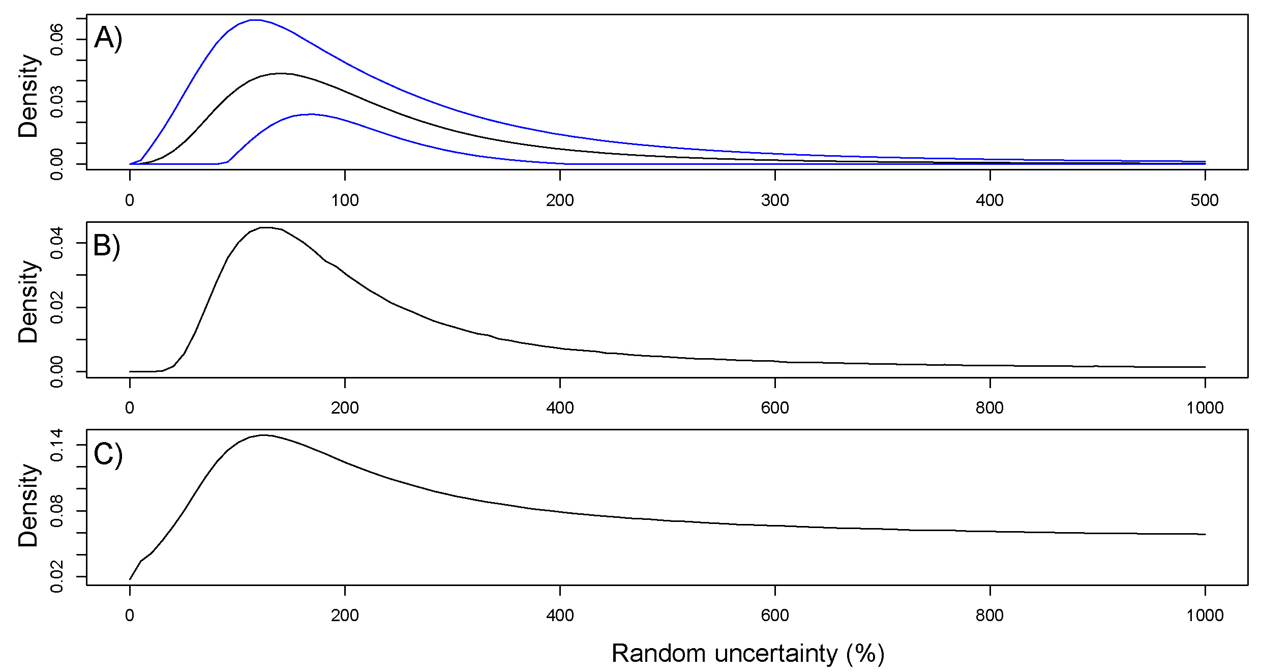
The constructed PDF for loess (PDF![]() , Fig.2A) is assumed to be representative only for fine grain OSL quartz ages from loess and loess-palaeosol sequences, and may exclusively be used for such environmental archives. More or different data used for future inverse modelling approaches may modify results, and therefore also results of age-depth models based on this PDF. Here we set the maximum percentage of random uncertainty to 100 %. However, if the OSL uncertainty is systematically underestimated, also higher percentages should be used. Such a possibility is explored by setting the maximal random uncertainty to 1000 %, along with an artificial dataset where random uncertainty is explored up to 500 % (Fig. 5). A maximum in the random part of uncertainty is located at 120 % for both PDFs. Because the method tends to underestimate random uncertainty, and also systematic uncertainty can be expected (e.g., Constantin et al. 2015), these results point at an even larger underestimation of uncertainty in the analysed luminescence datasets. A closer investigation in this direction is, however, clearly not aim of this manuscript, but may lie in the integration of the time dependent water content since deposition.
, Fig.2A) is assumed to be representative only for fine grain OSL quartz ages from loess and loess-palaeosol sequences, and may exclusively be used for such environmental archives. More or different data used for future inverse modelling approaches may modify results, and therefore also results of age-depth models based on this PDF. Here we set the maximum percentage of random uncertainty to 100 %. However, if the OSL uncertainty is systematically underestimated, also higher percentages should be used. Such a possibility is explored by setting the maximal random uncertainty to 1000 %, along with an artificial dataset where random uncertainty is explored up to 500 % (Fig. 5). A maximum in the random part of uncertainty is located at 120 % for both PDFs. Because the method tends to underestimate random uncertainty, and also systematic uncertainty can be expected (e.g., Constantin et al. 2015), these results point at an even larger underestimation of uncertainty in the analysed luminescence datasets. A closer investigation in this direction is, however, clearly not aim of this manuscript, but may lie in the integration of the time dependent water content since deposition.
A direct comparison to the information on the systematic and random uncertainty, as given by Constantin et al. (2014), is difficult in detail because of their deterministically set percentage versus the PDFs derived by our approach. A dominance of systematic uncertainty as proposed by Constantin et al. (2014) is possible, given that the PDF from the dataset by Constantin et al. (2014, see Fig. 6) allows for all possible uncertainty percentages. However, the proposed approach results in highest probabilities for random uncertainty of 120 %.
The increase in precision due to the Bayesian Prior of superposition is related to the amount of random uncertainty. The higher the random uncertainty, the higher is the improvement by the statistical method. The age recalculation removed all age inversions inherent to the initial dataset when considering the mean ages. However, more important are the changes of the age-depth relationship between 1 m and 3 m depth and the increase in the accumulation rate between 3 m and 4 m depth (Fig. 4). The recalculated dataset now reveals up to four different phases of sedimentation: (1) 0-1.5 m, (2) 1.5-3 m, (3) 3-4 m and (4) 4-8 m. Phases of rapid sedimentation (2 and 4) are linked to the corresponding loess layers. The recalculated results are not changing the palaeonvironmental interpretation by Kreutzer et al. (2012), however, they more sharply reveal the significance of the sedimentation phases. In combination with other datasets, this outcome has potential to further constraining the European climate history. Nevertheless, our results also show the limitation of our approach: The improvement of a single dataset does not necessarily lead to a changed palaeoenviromental history.
|
The application of a simulation allows only stratigraphically consistent data in a statistically justified way. Separating random and systematic uncertainty for luminescence data, can advance the precision of chronologies without decisively increasing precision in unjustified ways as specifically assuming uncertainty to be fully random. The accuracy depends on the systematic part of data uncertainty. We presume that all datasets with overlapping probability density functions of ages can be improved this way. The degree of data improvement depends on the shape of the PDF, the amount of overlap of age uncertainties and the number of measured ages of the chronology. The differentiation of clustered ages and/or hiatuses obvious from lithology is useful, and can be incorporated in algorithms, as available in the OxCal software (e.g., Bronk Ramsey, (1995) or ChronoModel (http://www.chronomodel.fr; manual: Vibet et al., 2016).
A more comprehensive database for a PDF![]() would be advantageous. However, more important would be the generation of decisively large datasets for single sediment sections. Unfortunately, only a few sections appear to be dated with the sufficient high resolution (e.g., at least every 50 cm; if stratigraphically applicable). We aim at finding a balance between the number and size of datasets and the needed constraints to generate reliable output. Regardless of whatever input PDF is used, resampling specific datasets will tend to show stratigraphically consistent results for a specific range of random and systematic uncertainty which may better explain a given dataset.
would be advantageous. However, more important would be the generation of decisively large datasets for single sediment sections. Unfortunately, only a few sections appear to be dated with the sufficient high resolution (e.g., at least every 50 cm; if stratigraphically applicable). We aim at finding a balance between the number and size of datasets and the needed constraints to generate reliable output. Regardless of whatever input PDF is used, resampling specific datasets will tend to show stratigraphically consistent results for a specific range of random and systematic uncertainty which may better explain a given dataset.
In contrast to calibrated ![]() C ages with complex PDF shapes, the OSL data used here are assumed to be normal distributed around a mean. This normal distribution has the advantage that improbable data structures do not need to be considered outliers. Other and more complex distributions and also density functions may be used in adjusted computer code, but are not commonly reported for luminescence ages. However, this also limits the increase in precision by applying Bayesian methods to luminescence dates.
C ages with complex PDF shapes, the OSL data used here are assumed to be normal distributed around a mean. This normal distribution has the advantage that improbable data structures do not need to be considered outliers. Other and more complex distributions and also density functions may be used in adjusted computer code, but are not commonly reported for luminescence ages. However, this also limits the increase in precision by applying Bayesian methods to luminescence dates.
Dating techniques relying on standards and constants have an overall uncertainty with parts of uncertainty being systematic and parts being random. Tests with synthetic data showed that datasets comprising a low number of ages lead to PDFs allowing for systematic and random uncertainty in the whole range between 0 % and 100 %. In cases where the amount of random/systematic uncertainty is unknown, we suggest to conservatively draw random/systematic uncertainty from a uniform PDF from 0 % to 100 % or use dataset-specific PDFs once these are generated or compiled from the literature. Higher systematic uncertainties lead to relatively imprecise results of Bayesian age depth-models and vice versa.
|
With our approach, the random and systematic parts of uncertainty are not strictly separated for every single age, but a PDF is modelled for all ages; either of one data set or a suite of data sets with comparable genetic constraints. This approach may systematically fail to hit the correct random and systematic uncertainty parts for individual dates, but is a generalisation made to adequately describe a data set. Likewise, a dataset with a small number of ages will not generate a narrow PDF. However, since the amount of random and systematic parts of uncertainty can be different for individual dates of a chronology, we do not consider imprecise PDFs as problematic, but rather a realistic case. Moreover, especially PDFs resulting from short chronologies should be regarded carefully when the uncertainty is expected to be dominantly systematic. Finally, Bayesian age models are expected to produce results with an improved precision, in comparison to the original data. Nevertheless, this precision may become misleading if potential systematic uncertainties have been not included by the individual dates (or dating methods; e.g. systematically higher or lower water content than assumed for luminescence). Further, computation results should be interpreted as a result of the applied method, and not necessarily as a perfect estimate of the true precisions; see Bronk Ramsey, (2000) for a thorough discussion of what Bayesian ages stand for. Though the choice of a uniform Bayesian prior distribution is applied here, it is neither the only option (Bronk Ramsey, 2000; 2009), nor may it be in all cases the preferred one (e.g., Bronk Ramsey, 2000). However, it may be assumed as the most appropriate option if no additional information on this distribution is available. Independent determination of the minimum and maximum systematic (or random) uncertainty for luminescence data derived from physical processes (as e.g., decay constants) would be beneficial for future work, and has the potential to improve on the here presented PDFs by setting the limits parameter in the function recalculate.ages.
Using a combination of an inverse modelling approach to estimate the random and systematic parts of OSL data uncertainty and a Bayesian age-depth model, we increase the precision of fine grain quartz OSL chronologies. Where separation of uncertainty into random and systematic parts is impossible, we propose to use a uniform PDF allowing for random uncertainty between 0 % and 100 %. Exemplary the precision of ages has been improved by 21-30 %, depending on the PDF used for random/systematic uncertainty. The applied approach of separating uncertainty parts of luminescence data may be applied to other environmental archives such as fluvial, limnic and marine datasets, and to other (luminescence) dating techniques. The application of the presented approach leads to a higher precision of luminescence-based chrono-stratigraphies, allowing more detailed conclusions about the timing and duration of Earth surface dynamics as preserved by sedimentological records.
Implementation of the approach using free and open software allows for a maximum of transparency and reproducibility. Adaptation of the provided functions for and application to new data sets (other OSL measurement protocols and techniques, other dosimeters, etc.) is encouraged and shall result in an active discussion of uncertainty patterns across these data sets.
This investigation was carried out in the context of the CRC 806 ''Our way to Europe``, supported by the DFG [Deutsche Forschungsgemeinschaft, grant number INST 216/596-2]. The work of SK is financed by a programme supported by the ANR - n![]() ANR-10-LABX-52. CZ is supported by a PSL fellowship. We thank Frank Preusser and two anonymous reviewers for constructive editorial work and for their valuable comments improving this manuscript.
ANR-10-LABX-52. CZ is supported by a PSL fellowship. We thank Frank Preusser and two anonymous reviewers for constructive editorial work and for their valuable comments improving this manuscript.
Agterberg, F.P., Hammer, O., Gradstein, F.M., 2012. Chapter 14 - Statistical Procedures, in: Gradstein, F.M., Ogg, J.G., Schmitz, M.D., Ogg, G.M. (Eds.), The Geologic Time Scale. Elsevier, Boston, pp. 269-273.
Aitken, M.J., 1998. Introduction to optical dating: the dating of Quaternary sediments by the use of photon-stimulated luminescence. Clarendon Press.
Aitken, M.J., 1985. Thermoluminescence dating. Academic Press.
Bayliss, A., Ramsey, C.B., 2004. Pragmatic Bayesians: a Decade of Integrating Radiocarbon Dates into Chronological Models, in: Buck, C.E., Millard, A.R. (Eds.), Tools for Constructing Chronologies, Lecture Notes in Statistics. Springer London, pp. 25-41.
Blaauw, M., 2010. Methods and code for ''classical`` age-modelling of radiocarbon sequences. Quaternary Geochronology 5, 512-518. doi:10.1016/j.quageo.2010.01.002
Blaauw, M., Christen, J.A., 2011. Flexible paleoclimate age-depth models using an autoregressive gamma process. Bayesian Anal. 6, 457-474. doi:10.1214/ba/1339616472
Blaauw, M., Heegaard, E., 2012. Estimation of Age-Depth Relationships, in: Birks, H.J.B., Lotter, A.F., Juggins, S., Smol, J.P. (Eds.), Tracking Environmental Change Using Lake Sediments, Developments in Paleoenvironmental Research. Springer Netherlands, pp. 379-413.
Blockley, S.P.E., Blaauw, M., Bronk Ramsey, C., van der Plicht, J., 2007. Building and testing age models for radiocarbon dates in Lateglacial and Early Holocene sediments. Quaternary Science Reviews 26, 1915-1926. doi:10.1016/j.quascirev.2007.06.007
Blockley, S.P.E., Lowe, J.J., Walker, M.J.C., Asioli, A., Trincardi, F., Coope, G.R., Donahue, R.E., 2004. Bayesian analysis of radiocarbon chronologies: examples from the European Late-glacial. J. Quaternary Sci. 19, 159-175. doi:10.1002/jqs.820
Bronk Ramsey, C., 2009. Bayesian Analysis of Radiocarbon Dates. Radiocarbon 51, 337-360.
Bronk Ramsey, C., 2001. Development of the radiocarbon calibration program. Radiocarbon 43, 355-363.
Bronk Ramsey, C., 2000. Comment on ''The use of Bayesian Statistics for ![]() C Dates of Chronologically ordered samples: A Critical Analysis.`` Radiocarbon 42, 199-202.
C Dates of Chronologically ordered samples: A Critical Analysis.`` Radiocarbon 42, 199-202.
Bronk Ramsey, C., 1995. Radiocarbon calibration and analysis of stratigraphy. The OxCal program. Radiocarbon 37, 425-430.
Buck, C.E., Cavanagh, G., Litton, C., 1996. Bayesian Approach to Intrepreting Archaeological Data. Wiley.
Buck, C.E., Kenworthy, J.B., Litton, C.D., Smith, A.F.M., 1991. Combining Archaeological and Radiocarbon Information . A Bayesian Approach to Calibration. Antiquity 65, 808-821.
Buck, C.E., Litton, C.D., Smith, A.F.M., 1992. Calibration of radiocarbon results pertaining to related archaeological events. Journal of Archaeological Science 19, 497-512. doi:10.1016/0305-4403(92)90025-X
Buggle, B., Hambach, U., Glaser, B., Gerasimenko, N., Marković, S., Glaser, I., Zöller, L., 2009. Stratigraphy, and spatial and temporal paleoclimatic trends in Southeastern/Eastern European loess-paleosol sequences. Quaternary International 196, 86-106. doi:10.1016/j.quaint.2008.07.013
Buylaert, J.-P., Vandenberghe, D., Murray, A.S., Huot, S., De Corte, F., Van den Haute, P., 2007. Luminescence dating of old (> 70ka) Chinese loess: A comparison of single-aliquot OSL and IRSL techniques. Quaternary Geochronology 2, 9-14.
Chapot, M.S., Roberts, H.M., Duller, G.A.T., Lai, Z.P., 2012. A comparison of natural- and laboratory-generated dose response curves for quartz optically stimulated luminescence signals from Chinese Loess. Radiation Measurements 47, 1045-1052. doi:10.1016/j.radmeas.2012.09.001
ChongYi, E., Lai, Z., Sun, Y., Hou, G., Yu, L., Wu, C., 2012. A luminescence dating study of loess deposits from the Yili River basin in western China. Quaternary Geochronology 10, 50-55. doi:10.1016/j.quageo.2012.04.022
Combès, B., Philippe, A., 2017. Bayesian analysis of individual and systematic multiplicative errors for estimating ages with stratigraphic constraints in optically stimulated luminescence dating. Quaternary Geochronology 39, 24-34.
Constantin, D., Begy, R., Vasiliniuc, S., Panaiotu, C., Necula, C., Codrea, V., Timar-Gabor, A., 2014. High-resolution OSL dating of the Costineşti section (Dobrogea, SE Romania) using fine and coarse quartz. Quaternary International 334-335, 20-29. doi:10.1016/j.quaint.2013.06.016
Constantin, D., Camenita, A., Panaiotu, C., Necula, C., Codrea, V., Timar-Gabor, A., 2015. Fine and coarse-quartz SAR-OSL dating of Last Glacial loess in Southern Romania. Quaternary International 357, 33-43. doi:10.1016/j.quaint.2014.07.052
de Vleeschouwer, D., Parnell, A.C., 2014. Reducing time-scale uncertainty for the Devonian by integrating astrochronology and Bayesian statistics. Geology 42, 491-494. doi:10.1130/G35618.1
Fuchs, M., Kreutzer, S., Rousseau, D.-D., Antoine, P., Hattè, C., Lagroix, F., Moine, O., Gauthier, C., Svoboda, J., Lisá, L., 2013. The loess sequence of Dolní Vĕstonice, Czech Republic: A new OSL-based chronology of the Last Climatic Cycle: Loess sequence of Dolní Vĕstonice, Czech Republic: OSL chronology. Boreas 42, 664-677. doi:10.1111/j.1502-3885.2012.00299.x
Gelman, A., Carlin, J.B., Stern, H.S., Rubin, D.B., 2014. Bayesian data analysis. Chapman & Hall/CRC Boca Raton, FL, USA.
Gradstein, F.M., Ogg, J.G., Smith, A.G., 2004. A Geologic Time Scale 2004. Cambridge University Press.
Hercman, H., Gasiorowski, M., Pawlak, J., 2014. Testing the MOD-AGE chronologies of lake sediment sequences dated by the 210Pb method. Quaternary Geochronology 22, 155-162. doi:10.1016/j.quageo.2014.01.001
Hercman, H., Pawlak, J., 2012. MOD-AGE: An age-depth model construction algorithm. Quaternary Geochronology 12, 1-10. doi:10.1016/j.quageo.2012.05.003
Huntriss, A., 2008. A Bayesian analysis of luminescence dating (Thesis, NonPeerReviewed).
Kreutzer, S., Fuchs, M., Meszner, S., Faust, D., 2012. OSL chronostratigraphy of a loess-palaeosol sequence in Saxony/Germany using quartz of different grain sizes. Quaternary Geochronology 10, 102-109. doi:10.1016/j.quageo.2012.01.004
Lanos, P., Goff, M.L., Kovacheva, M., Schnepp, E., 2005. Hierarchical modelling of archaeomagnetic data and curve estimation by moving average technique. Geophys. J. Int. 160, 440-476. doi:10.1111/j.1365-246X.2005.02490.x
Lomax, J., Fuchs, M., Preusser, F., Fiebig, M., 2014. Luminescence based loess chronostratigraphy of the Upper Palaeolithic site Krems-Wachtberg, Austria. Quaternary International 351, 88-97. doi:10.1016/j.quaint.2012.10.037
Lu, Y.C., Wang, X.L., Wintle, A.G., 2007. A new OSL chronology for dust accumulation in the last 130,000 yr for the Chinese Loess Plateau. Quaternary Research 67, 152-160. doi:10.1016/j.yqres.2006.08.003
Meszner, S., Kreutzer, S., Fuchs, M., Faust, D., 2013. Late Pleistocene landscape dynamics in Saxony, Germany: Paleoenvironmental reconstruction using loess-paleosol sequences. Quaternary International, Closing the gap - North Carpathian loess traverse in the Eurasian loess belt 6th Loess Seminar, Wrocław, Poland Dedicated to Prof. Henryk Maruszczak 296, 94-107. doi:10.1016/j.quaint.2012.12.040
Meyers, S.R., Siewert, S.E., Singer, B.S., Sageman, B.B., Condon, D.J., Obradovich, J.D., Jicha, B.R., Sawyer, D.A., 2012. Intercalibration of radioisotopic and astrochronologic time scales for the Cenomanian-Turonian boundary interval, Western Interior Basin, USA. Geology 40, 7-10. doi:10.1130/G32261.1
Millard, A.R., 2006a. Bayesian analysis of ESR dates, with application to Border Cave. Quaternary Geochronology 1, 159-166. doi:10.1016/j.quageo.2006.03.002
Millard, A.R., 2006b. Bayesian Analysis of Pleistocene Chronometric Methods. Archaeometry 48, 359-375. doi:10.1111/j.1475-4754.2006.00261.x
Millard, A.R., 2004. Taking Bayes Beyond Radiocarbon: Bayesian Approaches to Some Other Chronometric Methods, in: Buck, C.E., Millard, A.R. (Eds.), Tools for Constructing Chronologies, Lecture Notes in Statistics. Springer London, pp. 231-248.
Mundil, R.,Ludwig K.R., Metcalfe I., Renne P.R., 2004. Age and Timing of the Permian Mass Extinctions: U/Pb Dating of Closed-System Zircons. Science 305, 1760-1763. doi:10.1126/science.1101012
Murray, A.S., Wintle, A.G., 2000. Luminescence dating of quartz using an improved single-aliquot regenerative-dose protocol. Radiation Measurements 32, 57-73. doi:10.1016/S1350-4487(99)00253-X
Preusser, F., Degering, D., Fuchs, M., Hilgers, A., Kadereit, A., Klasen, N., Krbetschek, M., Richter, D., Spencer, J.Q.G., 2008. Luminescence dating: basics, methods and applications. Eiszeitalter & Gegenwart/Quaternary Science Journal 57, 95-149. doi:10.3285/eg.57.1-2.5
R Develeopment Core Team, 2017. R: A Language and Environment for Statistical Computing. http://r-project .org
Rhodes, E.J., Bronk Ramsey, C., Outram, Z., Batt, C., Willis, L., Dockrill, S., Bond, J., 2003. Bayesian methods applied to the interpretation of multiple OSL dates: high precision sediment ages from Old Scatness Broch excavations, Shetland Isles. Quaternary Science Reviews, LED 2002 22, 1231-1244. doi:10.1016/S0277-3791(03)00046-5
Roberts, H.M., 2008. The development and application of luminescence dating to loess deposits: a perspective on the past, present and future. Boreas 37, 483-507. doi:10.1111/j.1502-3885.2008.00057.x
Rousseau, D.-D., Sima, A., Antoine, P., Hatté, C., Lang, A., Zöller, L., 2007. Link between European and North Atlantic abrupt climate changes over the last glaciation. Geophys. Res. Lett. 34, L22713. doi:10.1029/2007GL031716
Sageman, B.B., Singer, B.S., Meyers, S.R., Siewert, S.E., Walaszczyk, I., Condon, D.J., Jicha, B.R., Obradovich, J.D., Sawyer, D.A., 2014. Integrating 40Ar/39Ar, U-Pb, and astronomical clocks in the Cretaceous Niobrara Formation, Western Interior Basin, USA. Geological Society of America Bulletin B30929.1. doi:10.1130/B30929.1
Schnepp, E., Lanos, P., 2005. Archaeomagnetic secular variation in Germany during the past 2500 years. Geophys. J. Int. 163, 479-490. doi:10.1111/j.1365-246X.2005.02734.x Scholz, D., Hoffmann, D.L., 2011. StalAge - An algorithm designed for construction of speleothem age models. Quaternary Geochronology 6, 369-382. doi:10.1016/j.quageo.2011.02.002
Steier, P., Rom, W., 2000. The use of Bayesian statistics for ![]() C dates of chronologically ordered samples : A critical analysis. Radiocarbon 42, 183-198.
C dates of chronologically ordered samples : A critical analysis. Radiocarbon 42, 183-198.
Telford, R.J., Heegaard, E., Birks, H.J.B., 2004. All age-depth models are wrong: but how badly? Quaternary Science Reviews 23, 1-5. doi:10.1016/j.quascirev.2003.11.003
Timar-Gabor, A., Vandenberghe, D.A.G., Vasiliniuc, S., Panaoitu, C.E., Panaiotu, C.G., Dimofte, D., Cosma, C., 2011. Optical dating of Romanian loess: A comparison between silt-sized and sand-sized quartz. Quaternary International, The Second Loessfest (2009) 240, 62-70. doi:10.1016/j.quaint.2010.10.007
Trandafir, O., Timar-Gabor, A., Schmidt, C., Veres, D., Anghelinu, M., Hambach, U., Simon, S., 2015. OSL dating of fine and coarse quartz from a Palaeolithic sequence on the Bistrița Valley (Northeastern Romania). Quaternary Geochronology, LED14 Proceedings 30, Part B, 487-492. doi:10.1016/j.quageo.2014.12.005
Újvári, G., Kovács, J., Varga, G., Raucsik, B., Marković, S.B., 2010. Dust flux estimates for the Last Glacial Period in East Central Europe based on terrestrial records of loess deposits: a review. Quaternary Science Reviews 29, 3157-3166. doi:10.1016/j.quascirev.2010.07.005
Vibet, M.A., Philippe, A., Lanos, P., Dufresne, P., 2016. ChronoModel V1. 5 User’s manual. URL http://www. chronomodel.fr.
Wintle, A.G., 1973. Anomalous fading of thermo-luminescence in mineral samples. Nature 245, 143-144.